
Als Teil der Volvo Gruppe verkauft Volvo Trucks mittels einiger Kooperationen und Tochterfirmen weltweit LKWs. Auf seiner Internetseite gibt das Unternehmen im Bereich Investors Relations auch die Auftragseingänge und Abssatzzahlen pro Quartal bekannt. Anbei der Verlauf der Absatzzahlen. Der Einbruch in 2020 aufgrund der wirtschaftlichen Lage infolge der Corona-Epidemie ist deutlich sichtbar.


Periodische Effekte
Erster Schritt ist es, die Zeitreihe - in unserem Fall der Gesamtabsatz - näher kennenzulernen. Mit dem Seasonal Plot (plot 2) können wir die periodischen Effekte der Quartale betrachten. Dafür wird jedes Jahr als eigene Linie über die Quartale hinweg visualisiert. Die Darstellung erlaubt es saisonale Muster zu erkennen - auffällig ist hier die jeweilige Zunahme zum vierten Quartal - aber auch zur Identifikation von Jahren, die aus diesem Muster ausbrechen - dies könnte evtl. bei 2020 der Fall sein.
Auch der Seasonal Subseries Plot (plot 3) zeigt diese Effekte, allerdings sind nun die Quartale mit dem Verlauf über die Jahre hinweg abgebildet. Es zeigt sich, dass die Verkaufszahlen über alle Quartale hinweg bereits vor Corona abnahmen. Die blaue Linie - der Durchschnitt pro Quartal - zeigt auch hier den Anstieg hin zum vierten Quartal.
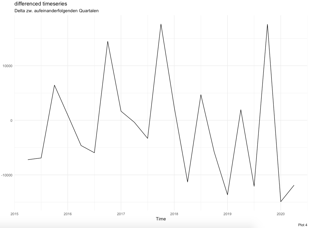
Plot 4 zeigt die Zu-/Abnahme zwischen den aufeinanderfolgenden Quartalen. Auch hier ist der Anstieg vom dritten zum vierten Quartal jeweils sichtbar. Es wird deutlich, dass 2019 einen anderen Verlauf nimmt.
Schließlich könnten wir noch versuchen, den Verlauf mittels logarithmischer Transformation zu begradigen. Einfachere Muster führen zu meist besseren Forecasts. Plot 5 zeigt bei unserer Zeitreihe keinen Effekt.
 |
 |
 |
 |


Training und Testdaten

Forecasting
Als erstes können wir die Zeitreihe mit simplen Methoden fortschreiben. Plot 8 zeigt, wie der meanf()-Befehl einfach den Durchschnitt der Periode fortschreibt. Von diesen simpleren Methoden gibt es einige, dargestellt in plot 10. Da sie keine Saisonalität berücksichtigen, habe ich sie anhand des Trainingsdatensets ohne Saisonalität trainiert. Ähnlich funktioniert die Methodik in Plot 11; hier habe ich eine lineare Regression hinterlegt, allerdings das Jahr 2019 als Wendepunkt hinterlegt. Die Fortschreibung in die Zukunft geschieht nur anhand des trainierten Modells mit den Daten ab 2019. Ähnlich funktioniert die Technik des Smoothings, aufgezeigt in Plot 12. Diese Forecasts sind fortgeschriebene Mittelwerte, bei welchen auf die letzten Werten am meisten Gewichtung gelegt wird. Plot 13 zeigt schließlich jene Methoden, welche auch die identifizierten periodischen Effekte fortführen können.
 |
 |
 |
 |
Validierung
Die Forecasts können wir nun dem Testdatensatz gegenüberstellen. In der Tabelle in Plot 14 sind verschiedene Indikatoren aufgeführt. Im Folgenden untersuche ich das Modell des Befehls stlf() genauer. Denn auch die Performance gegenüber dem Trainingsdatensatz müssen wir betrachten. Die folgenden Grafiken zeigen, dass das benutzte Modell die Rohdaten im Trainingsdatensatz relativ gut treffen und auch das Prediction Intervall ist aussagekräftig. |
 |
 |
 |
R Code
library(dplyr)
library(ggplot2)
library(reshape2)
library(zoo)
library(fpp2)
library(GGally)
library(seasonal)
library(viridis)
library(urca)

## Data Prep
data <- read.csv("~/Documents/Blog/19_Volvo units/Quarterly Orders.csv") %>%
  `colnames<-`(lapply(.[1, ], as.character)) %>%
  slice(10:13) %>%
  t(.) %>%
  `colnames<-`(lapply(.[1, ], as.character)) %>%
  .[-1, ] %>%
  as.data.frame() %>%
  mutate(period = rownames(.)) %>%
  mutate(period = paste(substr(period, start = 1, stop = 2),"/",substr(period, start = 3, stop = 4))) %>%
  mutate(period = as.yearqtr(period, format="%y / Q%q"))

## 1) individual time series
## 1a) analysing development
data <- data %>%
  `colnames<-`(c("Heavy-Duty", "Medium-Duty", "Light-Duty", "Total", "period")) %>%
  select("Heavy-Duty", "Medium-Duty", "Light-Duty", "Total") %>%
  mutate(`Heavy-Duty` = as.numeric(gsub(",","",`Heavy-Duty`))) %>%
  mutate(`Medium-Duty` = as.numeric(gsub(",","",`Medium-Duty`))) %>%
  mutate(`Light-Duty` = as.numeric(gsub(",","",`Light-Duty`))) %>%
  mutate(`Total` = as.numeric(gsub(",","",`Total`)))
data_ts <- ts(data, start=2015, frequency=4)
autoplot(data_ts) +
  theme_minimal() +
  labs(x = NULL, y = NULL, title = paste("Entwicklung der Bestellungen"), subtitle = ("von Volve Trucks weltweit"), caption = "Plot 1")
## 1b) analysing periodical effects
ggseasonplot(data_ts[,'Total'], year.labels=TRUE, year.labels.left=TRUE) +
  theme_minimal() + labs(title = paste("Seasonal plot"), caption = "Plot 2")
ggsubseriesplot(data_ts[,'Total']) +
  theme_minimal() + labs(y = NULL, title = paste("Seasonal subseries plot"), subtitle = ("blaue Linie = Durchschnitt pro Quartal"), caption = "Plot 3")
autoplot(diff(data_ts[,'Total'])) + #changes in the index
  theme_minimal() + labs(y = NULL, title = paste("differenced timeseries"), subtitle = ("Delta zw. aufeinanderfolgenden Quartalen"), caption = "Plot 4")
## 1c) BOX-COX TRANSFORMATIONS to make series more linear
lambda <- BoxCox.lambda(data_ts[,'Total'])
cbind(raw = data_ts[,'Total'], transform = BoxCox(data_ts[,'Total'], lambda)) %>% autoplot(facets = TRUE) +
  theme_minimal() + labs(title = paste("Seasonal plot"), subtitle = ("keine sichtbaren Effekte mit log-adjustment"), caption = "Plot 5")
## 1d) time series decomposition into trend-cycle, a seasonal and remainder component
data_ts[,'Total'] %>% decompose(type="additive") %>% autoplot() +
  theme_minimal() + labs(title = paste("classical additive decomposition"), subtitle = ("if seasonal fluctuations, or variation around trend-cycle not varying"))
data_ts[,'Total'] %>% decompose(type="multiplicative") %>% autoplot() +
  theme_minimal() + labs(title = paste("classical multiplicative decomposition"), subtitle = ("when variation in seasonal pattern or variation around trend-cycle"))
data_ts[,'Total'] %>% seas(x11="") %>% autoplot() +
  theme_minimal() + labs(title = paste("X11 decomposition"), subtitle = ("sophisticated methods for treating day variation & holiday effects"))
data_ts[,'Total'] %>% seas() %>% autoplot() +
  theme_minimal() + labs(title = paste("SEATS decomposition"), subtitle = ("works only with quarterly and monthly data"))
data_ts[,'Total'] %>%
  stl(t.window=12, s.window="periodic", robust=TRUE) %>% autoplot() + # t.window for trend (# of oberv. to use for estimating trend-cycle), s.window for season (# of years to estimate seasonal component) for how rapidly components can change; the smaller the faster
  theme_minimal() + labs(title = paste("STL decomposition"), subtitle = ("for any type of seasonality, robust to outliers"))
data_ts[,'Total'] %>% mstl() %>% autoplot() +
  theme_minimal() + labs(title = paste("automated STL decomp."), subtitle = ("with s.window=13 & t.window autom. for balancing overfitting & allowing slow change"), caption = "Plot 6")
# time series decomposition, plotting against raw data &
fit <- data_ts[,'Total'] %>% mstl()
autoplot(data_ts[,'Total'], series="Data") +
  autolayer(trendcycle(fit), series="Trend") +
  autolayer(seasadj(fit), series="Seasonally Adjusted") + #seasonal component removed
  scale_color_viridis(discrete=TRUE, direction=-1) +
  theme_minimal() + labs(x = NULL, y = NULL, title = paste("seasonally adjusted data"), subtitle = ("without seasonal component identified with automated STL decomp."), caption = "Plot 7")

## 2) training & testing data split
myts.train <- window(data_ts[,'Total'], end = c(2019,3))
myts.train_adj <- myts.train %>% mstl() %>%seasadj()
myts.test <- window(data_ts[,'Total'], start= c(2019,3))
autoplot(data_ts[,'Total']) +
  autolayer(myts.train, series="Training", size=1) +
  autolayer(myts.train_adj, series="Training seas. adj.") +
  autolayer(myts.test, series="Test", size=1) +
  scale_color_viridis(discrete=TRUE, direction=-1) +
  theme_minimal() + labs(x = NULL, y = NULL, title = paste("Trainings- & Testdatensatz"), caption = "Plot 8")

## 3) FORECASTING
# 3a) SIMPLE FORECASTING - ohne Berücksichtigung von Saisonalität
fc_simple1 <- meanf(myts.train_adj, h=5)
autoplot(myts.train, series="Training data") +
  autolayer(fc_simple1, series="meanf()", PI=FALSE) +
  autolayer(fitted(fc_simple1), series="meanf()") +
  scale_color_viridis(discrete=TRUE, direction=-1) +
  theme_minimal() + labs(x = NULL, y = NULL, title = paste("Funktionsweise der einfacheren Methoden"), subtitle = ("hier meanf()"),caption = "Plot 9")
fc_simple2 <- naive(myts.train_adj, h=5)
fc_simple3 <- naive(myts.train_adj, biasadj = TRUE, h=5)
fc_simple4 <- rwf(myts.train_adj, drift=TRUE, lambda=0, h=5, level=80) #forecast medians
fc_simple5 <- rwf(myts.train_adj, drift=TRUE, lambda=0, h=5, level=80, biasadj=TRUE) #forecast means
fc_simple6 <- croston(myts.train_adj, h=5)
fc_simple7 <- ses(myts.train_adj, h=5)
fc_simple8 <- holt(myts.train_adj, h=5)
fc_simple9 <- splinef(myts.train_adj, h=5)
fc_simple10 <- thetaf(myts.train_adj, h=5)
fc_simple11 <- forecast(myts.train_adj, h=5)
autoplot(myts.train) +
  autolayer(myts.train, series="Training", size=1) +
  autolayer(myts.train_adj, series="Training - seas. adj.") +
  autolayer(myts.test, series="Test") +
  autolayer(fc_simple1, series="meanf()", PI=FALSE) +
  autolayer(fc_simple2, series="naive()", PI=FALSE) +
  autolayer(fc_simple3, series="naive() - bias adj", PI=FALSE) +
  autolayer(fc_simple4, series="rwf()", PI=FALSE) +
  autolayer(fc_simple5, series="rwf() - bias adj.", PI=FALSE) +
  autolayer(fc_simple6, series="croston()", PI=FALSE) +
  autolayer(fc_simple7, series="ses", PI=FALSE) +
  autolayer(fc_simple8, series="holt", PI=FALSE) +
  autolayer(fc_simple9, series="splinef()", PI=FALSE) +
  autolayer(fc_simple10, series="thetaf()", PI=FALSE) +
  autolayer(fc_simple11, series="forecast()", PI=FALSE) +
  scale_color_viridis(discrete=TRUE, direction=-1) +
  theme_minimal() + labs(x = NULL, y = NULL, title = paste("simple Forecasting"), subtitle = ("ohne Berücksichtigung von Saisonalität"), caption = "Plot 10")
# 3b) PIECEWISE REGRESSION
h <- 5
time <- time(myts.train_adj)
time.break <- 2018
time.piece <- ts(pmax(0,time-time.break), start=2015)
time.new <- time[length(time)]+seq(h)
time_piece_new <- time.piece[length(time.piece)]+seq(h)
newdata <- cbind(time=time.new, time.piece = time_piece_new) %>% as.data.frame()
piecewise_linear <- tslm(myts.train_adj ~ time + time.piece)
fc_piecewise_linear <- forecast(piecewise_linear, newdata = newdata)
autoplot(myts.train) +
  autolayer(fitted(piecewise_linear), series="piecewise split") +
  autolayer(fc_piecewise_linear$mean, series="piecewise regression") +
  scale_color_viridis(discrete=TRUE, direction=-1) +
  theme_minimal() + labs(x = NULL, y = NULL, title = paste("piecewise regression"), caption = "Plot 11")
# 3c) SMOOTHING
fc_ses <- ses(myts.train_adj, h=5) #simple exponential smoothing (SES)
fc_holt1 <- holt(myts.train_adj,h=5) #holt-model to include trend
fc_holt2 <- holt(myts.train_adj,damped=TRUE, phi = 0.9, h=5) #damping usually btw. 0.8 and 0.9
autoplot(myts.train) +
  autolayer(myts.test, series="Test") +
  autolayer(fc_ses, series="simple exponential smoothing", PI=FALSE) +
  autolayer(fc_holt1, series="holt model", PI=FALSE) +
  autolayer(fc_holt2, series="holt model damped", PI=FALSE) +
  scale_color_viridis(discrete=TRUE, direction=-1) +
  theme_minimal() + labs(x = NULL, y = NULL, title = paste("Smoothing Methoden"), caption = "Plot 12")
# 3d) FORECASTING - mit Berücksichtigung von Saisonalität
fc_simple12 <- snaive(myts.train, h=5)
fc_simple13 <- stlf(myts.train, h=5) # stlf() decomp. via stl(), forecasting seas. adj. series, returning reaseason. fc
myts.train_adj2 <- myts.train %>% stl(t.window=5, s.window="periodic", robust=TRUE)
fc_simple14 <- forecast(myts.train_adj2, method="naive", h=5)
fc_decomp <- stlf(myts.train,lambda=BoxCox.lambda(myts.train),s.window=13,robust=TRUE,method="ets") %>% #STl to forecast seasonally adjusted series via mstl(), then reseasonalise forecasts
  forecast(h=5)
fc_hw_add <- hw(myts.train_adj,damped=FALSE,seasonal="additive", h=5) #holt & winter-model to include seasonality (additive for constant seasonal variations)
fc_hw_mult <- hw(myts.train_adj,damped=FALSE,seasonal="multiplicative", h=5) #holt & winter-model to include seasonality (multiplicative when growing/decreasing seasonal variation)
#summary(ets) #"AAN"/"MAN" - Holt´s linear method with additive/multiplicative errors //"AAN"/"MNN" - simple exponential smoothing with additive/multiplicative errors
autoplot(myts.train) +
  autolayer(myts.train, series="Training", size=1) +
  autolayer(myts.test, series="Test") +
  autolayer(fc_simple12, series="snaive()", PI=FALSE) +
  autolayer(fc_simple13, series="stlf()", PI=FALSE) +
  autolayer(fc_simple14, series="stl() & forecast()", PI=FALSE) +
  autolayer(fc_decomp, series="stlf()", PI=FALSE) +
  autolayer(fc_hw_add, series="holt & winter-model additive", PI=FALSE) +
  autolayer(fc_hw_mult, series="holt & winter-model multiplicative", PI=FALSE) +
  scale_color_viridis(discrete=TRUE, direction=-1) +
  theme_minimal() + labs(x = NULL, y = NULL, title = paste("Forecasting"), subtitle = ("mit Berücksichtigung der Saisonalität"), caption = "Plot 13")


##4 Validierung
# 4a) check against training data
validation <- rbind(
      round(accuracy(fc_simple1,myts.test),2)[2,],
      round(accuracy(fc_simple2,myts.test),2)[2,],
      round(accuracy(fc_simple3,myts.test),2)[2,],
      round(accuracy(fc_simple4,myts.test),2)[2,],
      round(accuracy(fc_simple5,myts.test),2)[2,],
      round(accuracy(fc_simple6,myts.test),2)[2,],
      round(accuracy(fc_simple7,myts.test),2)[2,],
      round(accuracy(fc_simple8,myts.test),2)[2,],
      round(accuracy(fc_simple9,myts.test),2)[2,],
      round(accuracy(fc_simple10,myts.test),2)[2,],
      round(accuracy(fc_simple11,myts.test),2)[2,],
      round(accuracy(fc_piecewise_linear, myts.test),2)[2,],
      round(accuracy(fc_ses, myts.test),2)[2,],
      round(accuracy(fc_holt1, myts.test),2)[2,],
      round(accuracy(fc_holt2, myts.test),2)[2,],
      round(accuracy(fc_simple12, myts.test),2)[2,],
      round(accuracy(fc_simple13, myts.test),2)[2,],
      round(accuracy(fc_simple14, myts.test),2)[2,],
      round(accuracy(fc_decomp, myts.test),2)[2,],
      round(accuracy(fc_hw_add, myts.test),2)[2,],
      round(accuracy(fc_hw_mult, myts.test),2)[2,]
      ) #find model with lowest scores for MAE, RMSE, MAPE, MASE
row.names(validation)<-c("meanf()","naive()","naive() - bias adj","rwf()","rwf() - bias adj.","croston()","ses",
                         "holt","splinef()","thetaf()","forecast()", "piecewise linear", "ses", "holt()", "holt() damped",
                         "snaive()","stlf()","stl() & forecast()", "stlf()", "holt&winter add", "holt&winter mult")
library(formattable)
formattable(as.data.frame(validation),
            list(`ME`= color_bar("#f5b7b1"),
                 `RMSE`= color_bar("#f5b7b1"),
                 `MAE`= color_bar("#f5b7b1"),
                 `MPE`= color_bar("#f5b7b1"),
                 `MAPE`= color_bar("#f5b7b1"),
                 `MASE`= color_bar("#f5b7b1"),
                 `ACF1`= color_bar("#f5b7b1"),
                 `Theil's U`= color_bar("#f5b7b1")
                 ), caption="plot 14 - validation")
# 4b) check against training data
autoplot(myts.train, series="training data") +
  autolayer(fitted(fc_simple13), series="stlf()") + #fitted values (predictions of y within the training-sample)
  autolayer(fc_simple13, series="stlf()", PI=TRUE) +
  autolayer(myts.test, series="test data") +
  scale_color_viridis(discrete=TRUE, direction=-1) +
  theme_minimal() + labs(x = NULL, y = NULL, title = paste("stlf() Forecasting"), caption = "Plot 15")
cbind(Data = myts.train, Fitted = fitted(fc_simple13)) %>% as.data.frame() %>%
  ggplot(aes(x=Data, y=Fitted)) +
  geom_point() +
  geom_abline(intercept=0, slope=1) +
  theme_minimal() + labs(x = NULL, y = NULL, title = paste("stlf() Forecasting"), subtitle = "1:1 Abbildung der Rohdaten durch Modell, wenn Punkte auf Linie", caption = "Plot 16")
checkresiduals(fc_simple13)  #goodness of fit in training sample
# > time plot: mean zero necessary & constant variance helpful
# > ACF plot: mean zero & no significant correlation necessary; above blue lines = correlations significant and autocorr.; trend -> large, positive autocorr. for small lags (nearby observations also nearby in size), slowly decreasing & seasonality -> autocorr. larger for seasonal lags
# > histogram of residuals: if not normally distr., prediction intervals computed with assumption of normal distribution may be inaccurate
# > Breusch-Godfrey/Ljung-Box test for regressions: small p-value = significant autocorrelation remaining, large values of Q = autocorr. not from white noise
cbind(Fitted = fitted(fc_simple13), Residuals=residuals(fc_simple13)) %>%
  as.data.frame() %>%
  ggplot(aes(x=Fitted, y=Residuals)) + geom_point() +
  theme_minimal() + labs(x = NULL, y = NULL, title = paste("stlf() Forecasting"), subtitle = "Heteroskedastizität, falls Muster erkennbar", caption = "Plot 17")