
Der Jahresabschluss 2019 der Daimler AG hat 350 teils eng beschriebene Seiten. Zur schnellen Analyse und ersten Einschätzung habe ich mir selbst ein PDF-Template zur Analyse von PDFs geschrieben (unten angehängt der R-Code) und aufbauend u.a. auf folgendem Intro wichtige Codes beschrieben.
Worthäufigkeiten
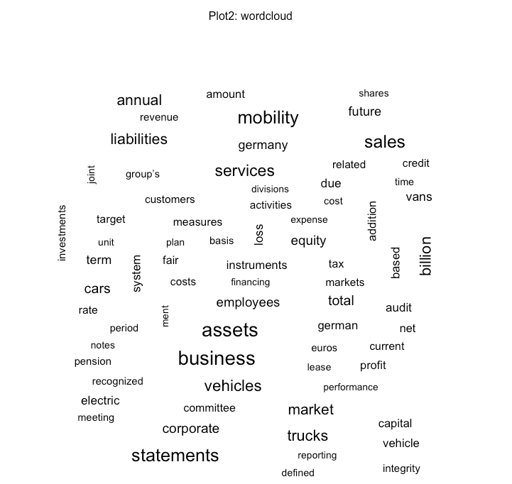
Zuerst schauen wir in Plot 1-4 nach den häufigsten Wörtern, bzw. Wortpaaren. Wir sehen die zu erwartenden Wörter eines Jahresabschlusses; aber auch spezifische Themen wie "Mobility" oder "Truck". Wir haben nun also bereits einen kleinen Einblick darin, was für Themen wichtig sein könnten.
 |
 |
 |
 |
 |
Sentiment
Was erfahren wir über die Stimmung - den Sentiment Score? Plot 5-13 zeigen uns verschiedenes dazu. Die Ausprägung von "positive" in Plot 5 lässt sich erklären. "Trust" auch; hier können wir aber tiefer tauchen und schauen, welche Wörter diese Ausprägung veranlassen. Genauso können wir schauen, welche Wörter in was für einem Umfang zur Stimmung beitragen. Doch wie sieht die Stimmung über das PDF hinweg aus? Plot 9 zeigt uns die Verteilung in Schritten von jeweils 80 Seiten. Wir sehen tatsächlich große Unterschiede zwischen den Schritten. Wo ist die Stimmung am schlechtesten? Die folgenden beiden Plots lassen vermuten, dass es hier um das Risiko-Kapitel geht und speziell Finanz- bzw. Währungsrisiken wichtig sind. Die Plots zum Maximum des Sentiment-Scores lassen vermuten, dass es hier um die Produkte geht.
 |
 |  |  |  |  |  |  |  |  |
Auch Themen können wir identifizieren (lassen); hier mit n=3. Allerdings wird noch nicht wirklich etwas erkennbar. Im Vergleich zwischen Topic1 und Topic2 können wir erahnen, dass es beim einen evtl. um Finanzthemen geht und beim anderen um Umweltstandards.
 |
 |
 |
Vergleich zu anderem Text
Wir können das PDF auch zu einem anderen PDF vergleichen. In diesem Fall ist text2 der Jahresabschluss 2019 der Deutschen Bank. In den Plots sehen wir in welchem Text Wörter häufiger benutzt werden, können die Gemeinsamkeit aber auch statistisch messen. Zudem können wir a) zwei Themen im zusammengefügten Text finden und b) testen, ob ein PDF auch jeweils ein Thema ergibt; also ob sich die PDFs thematisch so unterscheiden, dass dies erkennbar ist. Dies ist hier tatsächlich der Fall, wie wir im letzten Screenshot sehen können.
 |
 |
 |
 |
 |
 |
 |
Die nrc-Bibliothek zur Sentimentanalyse wird hier beschrieben:
Crowdsourcing a Word-Emotion Association Lexicon, Saif Mohammad and Peter Turney, Computational Intelligence, 29 (3), 436-465, 2013.
Emotions Evoked by Common Words and Phrases: Using Mechanical Turk to Create an Emotion Lexicon, Saif Mohammad and Peter Turney, In Proceedings of the NAACL-HLT 2010 Workshop on Computational Approaches to Analysis and Generation of Emotion in Text, June 2010, LA, California.
Emotions Evoked by Common Words and Phrases: Using Mechanical Turk to Create an Emotion Lexicon, Saif Mohammad and Peter Turney, In Proceedings of the NAACL-HLT 2010 Workshop on Computational Approaches to Analysis and Generation of Emotion in Text, June 2010, LA, California.
Und hier der Code für R:
library(pdftools)
library(SnowballC)
library(dplyr)

# Text einlesen und vorbereiten
text <- pdf_text("~/Documents/Blog/Textanalyse_Template/Daimler 2019.pdf") %>%
  readr::read_lines()
text <- data.frame(matrix(unlist(text), byrow=T),stringsAsFactors=FALSE)
text <- tibble::rowid_to_column(text, "line")
names(text) <- c("line", "text")
library(tidytext)
library(tm)
custom_stop_words <- bind_rows(tibble(word = c("miss","€", "daimler", "mercedesbenz", "report", "§", "mercedes", "benz", "ag"),
                                      lexicon = c("custom")),
                               stop_words) #hier anpassen
tidy_text <- text %>%
  unnest_tokens(word, text) %>%
  anti_join(custom_stop_words)
tidy_text<-tidy_text[-grep("\\b\\d+\\b", tidy_text$word),]  #Nummern entfernen

# Plot1: die häufigsten Wörter
library(ggplot2)
tidy_text %>%
  count(word, sort = TRUE) %>%
  top_n(20) %>% #hier anpassen
  mutate(word = reorder(word, n)) %>%
  ggplot(aes(word, n)) +
  geom_col() +
  xlab(NULL) +
  coord_flip() +
  ggtitle("Plot1: die häufigsten Wörter") +
  theme(plot.title = element_text(size = 10, hjust = 0.5))
# Plot2: wordcloud
library(wordcloud)
layout(matrix(c(1, 2), nrow=2), heights=c(1, 4))
par(mar=rep(0, 4))
plot.new()
text(x=0.5, y=0.5, "Plot2: wordcloud")
tidy_text %>%
  count(word) %>%
  with(wordcloud(word, n, max.words = 100)) +
  ggtitle("Plot2: wordcloud") +
  theme(plot.title = element_text(size = 10, hjust = 0.5))
# Plot3: die häufigsten Bigramme
library(tidyr)
bigrams <-text %>%
  unnest_tokens(bigram, text, token = "ngrams", n = 2) %>%
  separate(bigram, c("word1", "word2"), sep = " ") %>%
  filter(!word1 %in% custom_stop_words$word,
         !word2 %in% custom_stop_words$word) %>%
  drop_na(word1) %>%
  drop_na(word2) %>%
  unite(bigram, word1, word2, sep = " ")
bigrams<-bigrams[-grep("\\b\\d+\\b", bigrams$bigram),]
bigrams %>%
  count(bigram, sort = TRUE) %>%
  top_n(10) %>% #hier anpassen
  mutate(bigram = reorder(bigram, n)) %>%
  ggplot(aes(bigram, n)) +
  geom_col() +
  xlab(NULL) +
  coord_flip() +
  ggtitle("Plot3: die häufigsten Bigramme") +
  theme(plot.title = element_text(size = 10, hjust = 0.5))
# Plot 4: die häufigsten Trigramme
trigrams <- text %>%
  unnest_tokens(trigram, text, token = "ngrams", n = 3) %>%
  separate(trigram, c("word1", "word2", "word3"), sep = " ") %>%
  filter(!word1 %in% custom_stop_words$word,
         !word2 %in% custom_stop_words$word,
         !word3 %in% custom_stop_words$word) %>%
  drop_na(word1) %>%
  drop_na(word2) %>%
  drop_na(word3)
trigrams <- trigrams %>%
  unite(trigrams, word1, word2, word3, sep = " ")
trigrams<-trigrams[-grep("\\b\\d+\\b", trigrams$trigrams),]  #remove numbers
trigrams %>%
  count(trigrams, sort = TRUE) %>%
  top_n(10) %>% #hier anpassen
  mutate(trigrams = reorder(trigrams, n)) %>%
  ggplot(aes(trigrams, n)) +
  geom_col() +
  xlab(NULL) +
  coord_flip() +
  ggtitle("Plot 4: die häufigsten Trigramme") +
  theme(plot.title = element_text(size = 10, hjust = 0.5))

# Sentiment-Analyse
library(tidytext)
#get_sentiments("afinn") #assigns words with a score that runs between -5 and 5
#get_sentiments("bing") #categorizes words in a binary fashion into positive and negative categories
#get_sentiments("nrc") #LICENSE NEEDED - categorizes words in a binary fashion (“yes”/“no”) into categories of positive, negative, anger, anticipation, disgust, fear, joy, sadness, surprise, and trust
library(textdata)
# Plot 5: welche Emotionen werden angesprochen?
tidy_text %>%
  inner_join(get_sentiments("nrc")) %>%
  count(sentiment, sort=TRUE) %>%
  mutate(sentiment = reorder(sentiment, n)) %>%
  ggplot(aes(sentiment, n)) +
  geom_col() +
  xlab(NULL) +
  coord_flip() +
  ggtitle("Plot 5: welche Emotionen werden angesprochen?") +
  theme(plot.title = element_text(size = 10, hjust = 0.5))
# Plot 6: was für "trust"-Wörter gibt es?
tidy_text %>%
  inner_join(get_sentiments("nrc")%>%
               filter(sentiment == "trust")) %>% #positive, negative, anger, anticipation, disgust, fear, joy, sadness, surprise, and trust
  count(word, sort = TRUE) %>%
  top_n(10) %>% #hier anpassen
  mutate(word = reorder(word, n)) %>%
  ggplot(aes(word, n)) +
  geom_col() +
  xlab(NULL) +
  coord_flip() +
  ggtitle("Plot 6: was für trust-Wörter gibt es?") +
  theme(plot.title = element_text(size = 10, hjust = 0.5))
# Plot 7: die häufigsten positiv & negativ-konnotierten Wörter
bing_word_counts <- tidy_text %>%
  mutate(word = wordStem(word)) %>%
  inner_join(get_sentiments("bing")) %>%
  count(word, sentiment, sort = TRUE) %>%
  ungroup()
bing_word_counts %>%
  group_by(sentiment) %>%
  top_n(10) %>% #hier anpassen
  ungroup() %>%
  mutate(word = reorder(word, n)) %>%
  ggplot(aes(word, n, fill = sentiment)) +
  geom_col(show.legend = FALSE) +
  facet_wrap(~sentiment, scales = "free_y") +
  labs(y = "Contribution to sentiment",
       x = NULL) +
  coord_flip() +
  ggtitle("Plot 7: die häufigsten positiv & negativ-konnotierten Wörter") +
  theme(plot.title = element_text(size = 10, hjust = 0.5))
# Plot8: Comparison-Wordcloud positive vs negative Wörter
library(reshape2)
layout(matrix(c(1, 2), nrow=2), heights=c(1, 4))
par(mar=rep(0, 4))
plot.new()
text(x=0.5, y=0.5, "Plot8: Comparison-Wordcloud positive vs negative Wörter")
tidy_text %>%
  inner_join(get_sentiments("bing")) %>%
  count(word, sentiment, sort = TRUE) %>%
  acast(word ~ sentiment, value.var = "n", fill = 0) %>%
  comparison.cloud(colors = c("gray50", "gray80"),
                   max.words = 100)
# Plot9: die Entwicklung des Sentiment-Scores per 80-Zeilen
library(scales)
text_sentiment <- tidy_text %>%
  inner_join(get_sentiments("bing")) %>%
  count(index = line %/% 80, sentiment) %>% #ggfalls n anpassen
  spread(sentiment, n, fill = 0) %>%
  mutate(sentiment = positive - negative)
ggplot(text_sentiment, aes(index, sentiment)) +
  geom_col(show.legend = FALSE) +
  ggtitle("Plot9: die Entwicklung des Sentiment-Scores per 80-Zeilen") +
  theme(plot.title = element_text(size = 10, hjust = 0.5))
# Plot10: wo ist der Sentiment-Score am niedrigsten?
sentiment_min <- text_sentiment %>%
  top_n(-1) %>%
  select(index) * 80
tidy_text %>%
  filter(line >= sentiment_min$index & line < sentiment_min$index +80) %>%
  count(word, sort = TRUE) %>%
  top_n(20) %>% #hier anpassen
  mutate(word = reorder(word, n)) %>%
  ggplot(aes(word, n)) +
  geom_col() +
  xlab(NULL) +
  coord_flip() +
  ggtitle("Plot10: wo ist der Sentiment-Score am niedrigsten?") +
  theme(plot.title = element_text(size = 10, hjust = 0.5))
trigrams_min <- text %>%
  filter(line >= sentiment_min$index & line < sentiment_min$index +80) %>%
  unnest_tokens(trigram, text, token = "ngrams", n = 3) %>%
  separate(trigram, c("word1", "word2", "word3"), sep = " ") %>%
  filter(!word1 %in% custom_stop_words$word,
         !word2 %in% custom_stop_words$word,
         !word3 %in% custom_stop_words$word) %>%
  drop_na(word1) %>%
  drop_na(word2) %>%
  drop_na(word3)
trigrams_min <- trigrams_min %>%
  unite(trigrams, word1, word2, word3, sep = " ")
trigrams_min %>%
  count(trigrams, sort = TRUE) %>%
  head(n=20) %>% #hier anpassen
  mutate(trigrams = reorder(trigrams, n)) %>%
  ggplot(aes(trigrams, n)) +
  geom_col() +
  xlab(NULL) +
  coord_flip() +
  ggtitle("Plot11: wo ist der Sentiment-Score am niedrigsten?") +
  theme(plot.title = element_text(size = 10, hjust = 0.5))
# Plot12: wo ist der Sentiment-Score am höchsten?
sentiment_max <- text_sentiment %>%
  top_n(1) %>%
  select(index) * 80
tidy_text %>%
  filter(line >= sentiment_max$index & line < sentiment_max$index +80) %>%
  count(word, sort = TRUE) %>%
  top_n(20) %>% #hier anpassen
  mutate(word = reorder(word, n)) %>%
  ggplot(aes(word, n)) +
  geom_col() +
  xlab(NULL) +
  coord_flip() +
  ggtitle("Plot12: wo ist der Sentiment-Score am höchsten??") +
  theme(plot.title = element_text(size = 10, hjust = 0.5))
trigrams_max <- text %>%
  filter(line >= sentiment_max$index & line < sentiment_max$index +80) %>%
  unnest_tokens(trigram, text, token = "ngrams", n = 3) %>%
  separate(trigram, c("word1", "word2", "word3"), sep = " ") %>%
  filter(!word1 %in% custom_stop_words$word,
         !word2 %in% custom_stop_words$word,
         !word3 %in% custom_stop_words$word) %>%
  drop_na(word1) %>%
  drop_na(word2) %>%
  drop_na(word3)
trigrams_max <- trigrams_max %>%
  unite(trigrams, word1, word2, word3, sep = " ")
trigrams_max %>%
  count(trigrams, sort = TRUE) %>%
  head(n=20) %>%
  mutate(trigrams = reorder(trigrams, n)) %>%
  ggplot(aes(trigrams, n)) +
  geom_col() +
  xlab(NULL) +
  coord_flip() +
  ggtitle("Plot13: wo ist der Sentiment-Score am höchsten??") +
  theme(plot.title = element_text(size = 10, hjust = 0.5))

# Plot 14: Identifikaton von n Themen und aus welchen Wörtern diese bestehen
library(topicmodels)
texts_DTM <- tidy_text  %>%
  mutate(document = "text1") %>%
  count(document, word) %>%
  cast_dtm(document, word, n)
library(ldatuning)
result <- FindTopicsNumber(
  texts_DTM,
  topics = seq(from = 2, to = 10, by = 1),
  metrics = c("Griffiths2004", "CaoJuan2009", "Arun2010", "Deveaud2014"),
  method = "Gibbs",
  control = list(seed = 77),
  mc.cores = 2L,
  verbose = TRUE
)
FindTopicsNumber_plot(result) #%>% #get n from the plots
topics <- LDA(texts_DTM, k = 3, control = list(seed = 1234))  #hier anpassen
topics_prob <- tidy(topics, matrix = "beta")
topic_terms <- topics_prob %>%
  group_by(topic) %>%
  top_n(15, beta) %>% #hier anpassen
  ungroup() %>%
  arrange(topic, -beta)
topic_terms %>%
  mutate(term = reorder_within(term, beta, topic)) %>%
  ggplot(aes(term, beta, fill = factor(topic))) +
  geom_col(show.legend = FALSE) +
  facet_wrap(~ topic, scales = "free") +
  coord_flip() +
  scale_x_reordered()  +
  ggtitle("Plot 14: Identifikaton von n Themen und aus welchen Wörtern diese bestehen?") +
  theme(plot.title = element_text(size = 10, hjust = 0.5))
# Plot 15: Unterschied zwischen topic 1 und 2
beta_spread <- topics_prob %>%
  mutate(topic = paste0("topic", topic)) %>%
  spread(topic, beta) %>%
  filter(topic1 > .001 | topic2 > .001) %>%
  mutate(log_ratio = log2(topic2 / topic1)) ##ggfalls hier anpassen
beta_spread %>%
  mutate(contribution = log_ratio) %>%
  arrange(desc(abs(contribution))) %>%
  head(20) %>% #hier anpassen
  mutate(term = reorder(term, contribution)) %>%
  ggplot(aes(term, log_ratio, fill = log_ratio > 0)) +
  geom_col(show.legend = FALSE) +
  xlab("terms") +
  ylab("Sentiment value * number of occurrences") +
  coord_flip() +
  ggtitle("Plot 15: Unterschied zwischen topic 1 und 2") +
  theme(plot.title = element_text(size = 10, hjust = 0.5))


#Vergleich zu einem anderen PDF-Text
text2 <- pdf_text("~/Documents/Blog/Textanalyse_Template/Deutsche Bank 2019.pdf") %>%
  readr::read_lines()
text2 <- data.frame(matrix(unlist(text2), byrow=T),stringsAsFactors=FALSE)
text2 <- tibble::rowid_to_column(text2, "line")
names(text2) <- c("line", "text")
joined_texts <- bind_rows(text %>%
                            mutate(source = "text1"),
                          text2 %>%
                            mutate(source = "text2"))
tidy_texts <- joined_texts %>%
  unnest_tokens(word, text) %>%
  anti_join(custom_stop_words)
tidy_texts<-tidy_texts[-grep("\\b\\d+\\b", tidy_texts$word),]  #remove numbers

# Plot16: Vergleich der häufigsten Wörter
frequency <- tidy_texts %>% #
  group_by(source) %>%
  count(word, sort = TRUE) %>%
  left_join(tidy_texts %>%
              group_by(source) %>%
              summarise(total = n())) %>%
  mutate(freq = n/total)
frequency <- frequency %>%
  select(source, word, freq) %>%
  spread(source, freq) %>%
  arrange(text1, text2)
ggplot(frequency, aes(text1, text2)) +
  geom_jitter(alpha = 0.1, size = 2.5, width = 0.25, height = 0.25) +
  geom_text(aes(label = word), check_overlap = TRUE, vjust = 1.5) +
  scale_x_log10(labels = percent_format()) +
  scale_y_log10(labels = percent_format()) +
  geom_abline(color = "red") +
  ggtitle("Plot16: Vergleich der häufigsten Wörter") +
  theme(plot.title = element_text(size = 10, hjust = 0.5))
# Statist. Ähnlichkeit zwischen den beiden Texten nach Worthäufigkeit
cor.test(data = frequency[,],~ text1 + text2)
# Plot17: Wichtige Wörter, welche die beiden Texte im Vergleich ausmachen (nach Zipf`s Law)
texts_words <- tidy_texts %>%
  count(source, word, sort = TRUE) %>%
  ungroup()
tw_idf <- texts_words %>%
  bind_tf_idf(word, source, n) %>%
  arrange(desc(tf_idf))
tw_idf %>%
  arrange(desc(tf_idf)) %>%
  mutate(word = factor(word, levels = rev(unique(word)))) %>%
  group_by(source) %>%
  top_n(15) %>%  #hier anpassen
  ungroup() %>%
  ggplot(aes(word, tf_idf, fill = source)) +
  geom_col(show.legend = FALSE) +
  labs(x = NULL, y = "tf-idf") +
  facet_wrap(~source, ncol = 2, scales = "free") +
  coord_flip() +
  ggtitle("Plot17: Wichtige Wörter, welche die beiden Texte im Vergleich ausmachen (nach Zipf`s Law)") +
  theme(plot.title = element_text(size = 10, hjust = 0.5))

# Plot 18: zwei gemeinsame Themen in beiden Texten
texts_DTM <- tidy_texts %>%
  count(source, word) %>%
  cast_dtm(source, word, n)
topics <- LDA(texts_DTM, k = 2, control = list(seed = 1234))
topics_prob <- tidy(topics, matrix = "beta") #probability of that term being generated from that topic for each line
topic_terms <- topics_prob %>%
  group_by(topic) %>%
  top_n(10, beta) %>% #hier anpassen
  ungroup() %>%
  arrange(topic, -beta)
topic_terms %>%
  mutate(term = reorder_within(term, beta, topic)) %>%
  ggplot(aes(term, beta, fill = factor(topic))) +
  geom_col(show.legend = FALSE) +
  facet_wrap(~ topic, scales = "free") +
  coord_flip() +
  scale_x_reordered() +
  ggtitle("Plot 18: zwei gemeinsame Themen in beiden Texten") +
  theme(plot.title = element_text(size = 10, hjust = 0.5))
# plot 19: die größten Unterschiede zwischen beiden gemeinsamen Themen
beta_spread <- topics_prob %>%
  mutate(topic = paste0("topic", topic)) %>%
  spread(topic, beta) %>%
  filter(topic1 > .001 | topic2 > .001) %>%
  mutate(log_ratio = log2(topic2 / topic1))
beta_spread %>%
  mutate(contribution = log_ratio) %>%
  arrange(desc(abs(contribution))) %>%
  head(20) %>% #hier anpassen
  mutate(term = reorder(term, contribution)) %>%
  ggplot(aes(term, log_ratio, fill = log_ratio > 0)) +
  geom_col(show.legend = FALSE) +
  xlab("terms") +
  ylab("Sentiment value * number of occurrences") +
  coord_flip() +
  ggtitle("plot 19: die größten Unterschiede zwischen beiden gemeinsamen Themen") +
  theme(plot.title = element_text(size = 10, hjust = 0.5))
# gamma ist der Anteil an Wörtern, aus welchen jeweils ein Thema generiert wurde
# d.h. je mehr ein PDF ein Thema ausmacht, desto höher das Gamma
# -> thematischer Unterschied, wenn jeweils ein PDF zu einem Topic beiträgt
topic_documents <- tidy(topics, matrix = "gamma")
topic_documents